How to use the AIRS SkewT Visualization Tool

How to Use the AIRS SkewT Visualization Tool

This application generates SkewT-LogP diagrams based on air temperature and water vapor measurements derived from Atmospheric Infrared Sounder (AIRS) instrument, in conjunction with the Advanced Microwave Sounder Unit A (AMSU-A), aboard NASA's Aqua Earth climate study spacecraft (launched May 4, 2002). The program consists of a "smart" web page and an embedded Java applet, all of which operate entirely within the computer memory managed by your Internet browser program. Any recent version of the most popular browser programs (Netscape Navigator, Internet Explorer, Safari, Firefox, and Opera) should be adequate when run on the Windows XT, Macintosh, and UNIX/Linux platforms (Note: Internet Explorer on Macintosh is not supported). In addition, your browser must be enabled for Java and Javascript functionality. While every effort has been made to make the process efficient, the page loading times for your computer and browser may depend on your Internet connection and available memory.

To better understand how these instruments can observe a particular location on Earth let us first look at the way in which the Aqua spacecraft provides a platform for these observations from 705 km (438 miles) up in polar orbit. We will then describe the steps for identifying the time and location when these observations are available, typically twice a day for the past several days. With this understanding, you can then generate SkewT plot images within your Internet browser for any place on Earth (including your own backyard!)

Understanding the Aqua Spacecraft Orbit

Spacecraft circling the Earth all have an orbital path which can be imagined as a flat round disk with the Earth at its center (think of a phonograph record or a very large CD). This disk is usually tipped or inclined at an angle to the Earth's equator. For a Space Shuttle mission, this angle of tilt is anywhere from 28.5 degrees (straight east from the NASA Kennedy Space Center) up to 51.6 degrees (to get to the International Space Station). Many weather satellites, however, attempt to observe the entire surface of the Earth as it rotates by having an orbit that always passes over the polar regions. Therefore, at launch time this angle of inclination is increased to nearly 90 degrees. Instead of the image of the Earth with a disk wrapped around its belly, we now have the image of a wheel with the Earth at its axis. This is referred to as a polar orbit.

Because the Earth is not a perfectly round and homogeneous sphere, irregularities in its gravity field have a profound effect on orbits relatively close to the surface. These irregularities actually cause the orbital disk to slowly rotate about the vertical axis in a wobbling motion like a spinning top. The east-west motion of this precession can be imagined from the perspective of an observer riding atop the Aqua spacecraft as he looks out at the stars in space. For example, in a polar orbit coming up from the Equator and ready to fly over the North Pole, the observer looking straight ahead might see the stars of the Big Dipper. One orbit later, the observer looking ahead would see a different set of stars, this time slightly to the left of the Big Dipper. The rate of this precession is dependent on both the altitude and orbital inclination angle (with respect to the Equator). For the Aqua spacecraft, the orbit is inclined 98.2 degrees at an altitude of 705 km (438 miles). That is, the orbit is tipped up from the equator, past the North Pole and an additional 8.2 degrees over to the other side. Therefore, to an observer on the ground, Aqua appears to rise in the west and set in the east! This orbit, however, matches up with Earth's annual revolution around the Sun such that Aqua will always cross the Equator at 1:30 PM going north and 1:30 AM going over the Equator in a southerly direction. On each pass over the Equator a different location on the ground (i.e., longitude) will be down below, but the lighting conditions will always be the same. This cycle does repeat in a predictable manner such that the Aqua spacecraft will pass over any given spot (including your home!) exactly once every 16 days.

Identifying Opportunities for Ground Observations

Because the AIRS instrument looks down and scans the Earth horizon from right to left, each of these swaths is about 1,650 km (1,030 miles) wide. This polar orbit, combined with the Earth's rotation underneath the orbit, ensures that most every spot on the surface is observed at least twice per day. For example, at the NASA Jet Propulsion Laboratory near Los Angeles, California, AIRS observes this area every day around 4:00 PM and 4:00 AM local time. Latitudes closer to the poles are observed four or more times per day.

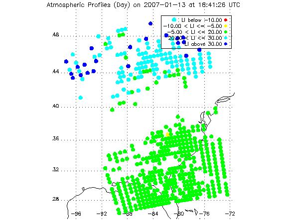
Consider the image shown below that depicts AIRS observations (merged with observations by AMSU-A) of the southeast United States in the late afternoon on January 17, 2007 (18:41:26 UTC is 1:41:26 PM local time). This data swath (about six minutes long) runs from south to north, scanning from left to right such that each colored circle represents one vertical column of air about 50 km (31 miles) in diameter. If 100% of the original data observations were shown, you would see a solid pattern of colored circles consisting of 45 "rows", each containing 30 footprints. In fact, due to turbulent weather and other difficulties in reconstructing a valid data set from all the observations, several footprints are not shown. Nonetheless, a full AIRS data set is equivalent to simultaneously releasing 1,350 weather balloons every six minutes, 24 hours a day for the past several years! This SkewT visualization tool, however, provides access to the observations for just the last several days of AIRS observations.

Still, a great deal of information can be deduced from this single six-minute data set. The circles are color-coded to convey the magnitude of a common weather-related indicator known as Lifted Index. A negative Lifted Index value indicates unstable (i.e., stormy) atmospheric conditions in the lower troposphere. The entire region across the Florida Peninsula and Panhandle, out to sea, are all at best neutrally stable. The data gap to the northwest may correspond to very irregular terrain (hills) and possibly a storm front, which is more difficult for AIRS to penetrate with infrared sensors. Farther inland, however, atmospheric conditions are decidedly more stable. When selecting an AIRS data set for a SkewT diagram, you will use this color coding, along with location, to examine data for one of these footprints at a time.

Procedure for Requesting AIRS Observations

Because the exact time that Aqua passes over a specific location is changing constantly over a 16-day cycle, the SkewT application will only be able to retrieve these ground tracks (called data granules) when you provide the following information:

Ground Track Selection Criteria

Latitude and Longitude You may specify the exact coordinates (if you know them) or simply use a clickable Earth map that has been provided. Remember, all longitudes west of the Prime Meridian (Greenwich, England) are negative numbers (e.g., Los Angeles is located at 34.05 degrees Latitude and -118.24 degrees Longitude).
Calendar Date or dates for which you wish to search for ground tracks containing the specified location. In a few rare occasions there may be a coverage gap for a particular location.
Lighting Conditions You may specify a preference for local lighting conditions as daytime only, nighttime only, or both daytime or nighttime conditions. Note that some ground tracks near the poles may have only daytime or nighttime conditions depending on the season.
Lat/Lon Granule Placement Because the above criteria will probably yield more than one matching granule ground track, you may wish to narrow the choice to either of the following choices that will produce one and only one match:

Show just the very latest six-minute data granule that contains the specified latitude/longitude and lighting conditions.
Show the one data granule in which the latitude/longitude position is closest to the middle of the ground track. This may be useful because the closer the specified point is to the middle of the ground track, the smaller the area that was scanned. For example, the instrument looking obliquely at a point at the far end of the scan (near the horizon) is collecting data over a much larger area than for a point straight below the spacecraft.

The simplest option, of course, is just to request all data granules that match the first three criteria and choose one data set for further study. The SkewT tool will allow you to flip through all the optional data sets before selecting a single footprint for a SkewT diagram.

This search process is fairly quick, perhaps five seconds for each date to be searched, so please be patient. A successful match with at least one available ground track will automatically transfer you to another page. If no matching results are found, you will be asked to return to the starting page to begin a new search.

On this new page click through the available ground track images (as shown earlier) and select one from which to build SkewT diagrams. Click the "Load Selected Ground Track" button and you will be transferred to another page.

You may always go back to STEP 1 by clicking on the "Reset Selections" button.

You are now ready to generate a SkewT diagram! This page may also take about 10 seconds to load into your browser. It contains not only a powerful Java applet to build the SkewT diagram, but also all data for each of the 1,350 footprints from the selected six-minute granule data set. Once this granule data set is loaded into your browser memory you do not even have to stay connected to our web site. You can simply save the current HTML page to your hard drive and open it again at any time with your browser program.

This final screen consists of two separate windows. In the first window is the ground track you have selected, along with a reminder of the other ground tracks that satisfied your original search criteria. In the ground track image, if you move the mouse over a circle, depending on your browser, you will see the latitude and longitude of that footprint. In addition, if you look at the bottom of your browser window, the status/message bar will also show a string of numbers and text indicating that the application is ready for you to click and generate a SkewT plot. Generating the SkewT diagram now is as easy as clicking on the appropriate footprint. Then, if you click on the actual SkewT image, you can also move the mouse over any portion of the figure and it will show you the corresponding temperature and pressure level.

This SkewT page will also explain how to copy the SkewT plot data to your own computer.

To plot any of the other profiles in the same granule data set, simply return to the ground track image and click on a different footprint circle. To look at the profile data from one of the other potential ground tracks, use the "BACK" button to return to the page before the SkewT window.

If you have not already read the previous section "What is a SkewT Diagram?", you may want to do so now.

You may always go back to STEP 1 by clicking on the "Reset Selection Criteria" button.